Arrays¶

Link with Playlist

One of the most basic composite data structure in computer science is the array. Understanding how arrays work and their associated algorithms is essential to understanding computer science.

In Python¶

Arrays are used extensively in Python. The following types have arrays in their core:

string
bytes and bytearray
tuple and list
set
dict

Definition¶

An array is an area of memory composed of zero or more same-sized elements. You can access an individual element in the array by calculating the offset given the size of each element and the index of the element in the array.

(Picture of an array, pointing with the finger. Add names as they are used.)

Some programming languages, like Python, use 0-based indexing. This means that the first element is the element at index 0. This makes calculating offsets ridiculously easy, but it conflicts with natural languages, which label the first element with number 1, not 0.

Other programming languages use 1-based indexing. This means that the first element is the element at index 1. This is preferrable because it maps well to natural languages. Mathematical notation typically uses 1-based indexing as well. IE, the first column is column 1, not 0. The key is that in calculating the offsets, you have to subtract 1 from the index.

Associated Algorithms¶

There are several algorithms that go hand-in-hand with arrays. There are also some techniques that have developed over the years to make working with arrays easier and faster.

Creating an Array¶

In order to create an array, you need to find a contiguous region of memory that is free to use. Sometimes you want to reserve extra space at the end of the array in anticipation of the array growing.

(Animation showing the program finding a free space of memory big enough for the array. There should be holes of various sizes.)

In terms of memory, it should be obvious that the array itself requires O(n) memory.

(Animation showing the size of the array.)

Some languages like C/C++ do not initialize the values in the array. It expects you will do that in due course. These languages give you O(1) creation of an array in time, but you’ll have to populate the elements yourself, which means it is not a big saving.

(Animation shows that the contents of the array is random.)

Most languages, including Python initialize the values to some value. For instance, when creating a list in Python, you have to tell it what the initial elements will be, and it will copy them over for you. This makes the complexity O(n) in time.

(Animation showing the elements copied over.)

Adding Elements¶

The algorithm to add elements is slightly different depending on where you want to add the element. However, no matter where you want the element to go, you first need to check that you have enough room for the new elements. If not, then the array must be copied to a region of memory with enough space for the new elements. The elements that are added can be added during the copy process.

(Animation showing the array being copied from one region of memory to another. There is a pointer to the beginning of the array that must move, as well as a designation of how much room to leave for the array. The old array is marked for deletion.)

If you add the elements to the end, and there is room for it, adding a single element is O(1) in time and memory. For multiple elements, O(n) in time and memory. n is the number of elements added.

If you add the elements to the beginning, then the entire array needs to be shifted. Each element needs to be copied to the next space over. This will take O(n) of time, where n is the number of elements in the array. It only requires O(1) of memory to copy all the elements, however.

(animation showing the elements shifting over.)

If you want to add elements to the middle, then only the elements after the added elements need to be shifted. We’ll call this O(n) in time and O(1) in memory. Remember, Big-O gives us an upper bound, not an average.

(Animation showing the elements shifting over.)

Adding Elements Repeatedly¶

Typically, you don’t know all the elements you want to add, or you want to build up the array over time. If you want to build up an array of n elements, and you naively only allocate enough memory for the new array, then you’d need to copy over every element into a new array, even if you were only adding elements to the end. This would lead to $1 + 2 + 3 + \dots + n$ copies, which is:

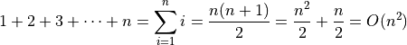
$1 + 2 + 3 + \dots + n = \sum_{i=1}^{n} i = \frac{n(n+1)}{2} = \frac{n^2}{2} + \frac{n}{2} = O(n^2)$

(As an aside, we can use proof by induction to solve this. See my Basic Mathematics video on that topic.)

This is really bad!

We might try to limit the number of copies by allocating extra memory. How much extra memory? If we only add a fixed number of extra space each time we copy, then we’ve not eliminated the $O(n^2)$ behavior.

If, instead, we doubled the amount of memory, then we can get a logarithmic number of copies. (Python uses 1.125 instead of 2 =- n+(n>>3).) This, combined with the relative rareness of the copies, means that we can add elements to the end of an array with an amortized cost of $O(1)$ . What “amortized” means is that while any individual addition may not be $O(1)$ , after adding many elements, it will be the same as $O(1)$ .

Let’s walk though the math behind this. Let’s say we increase the size of the array by $a$ every time we exceed the size of the array with our additional element. If we start with 1 elements, then the operations would be:

The first element creates a new array of size 1. Copies over the new value.
The second element creates a new array of size a. Copies of the one existing value and the new value.
The third element up to the a th element just adds the new element to the end. One more copy per element.
When we hit the a’th element, we have to create a new array of size $a^2$ . That involves a copies plus the new element.
We can simply add elements all the way up to $a^2$ . One copy each.
When we hit $a^2$ , then we need to create a new array of size $a^3$ and copy over $a^2$ elements. Then we add the new one.
After copying over $n$ elements, we have done exactly $\log_a n$ copies in addition to the $n$ copies to add things to the end. So we end up with the total:

$n + \sum_{i=1}^{\log_a n} a^i = n +\frac{1-a^{log_a n}}{1-a} = n+ \frac{1-n}{1-a} = O(n)$

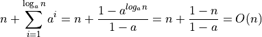
(Again, you can use proof by induction to prove the sum.)

Note that since adding $n$ elements takes $O(n)$ time, we say that each individual addition takes only $O(1)$ time amortized. Each individual add could take up to $O(n)$ time if it triggers a copy of the array, but doing this many times will give you the linear behavior, not the quadratic behavior.

Removing Elements¶

Removing elements works much like adding elements, except we don’t have to worry about there being enough room for all of the elements.

If we remove from the end, it is a simple $O(1)$ operation. Really, all we have to do is say that the array is now one element shorter. In Python, we need to tell the referenced object that it now has one fewer reference. Garbage collection is often considered separate from these algorithms.

If we remove elements from anywhere else, then we need to shift the elements down on top of the removed elements. This can be quite expensive. It is, in fact, O(n) in time, where n is the length of the array. It is O(1) in memory, however, since you only need to know the index you are copying from and the index you are copying to.

Finding Elements¶

Finding elements by index is very simple. It is always O(1) in time and memory. Just calculate the offset by multipying the index by the size of each element.

Finding elemetns by value is a little trickier. Remember that Big-O is the upper bound! If you’re looking for a particular element by its value, then you might be really unlucky and find it is the last element you looked at. You’d have looked at each element, in whatever pattern you want, whether thats from start to finish or from end to beginning, or some other algorithm. So finding it is O(n) in time but only O(1) in memory, since you can easily remember which elements you have already visited just by knowing how many you have seen so far.

Things get a little trickier if you want to find a sequence of elements by their value. Worst case, this can be O(mn), where m is the length of the sequence you are looking for and n is the length of the array. Of course, it would take a particularly diabolical array and comparing sequence to get this kind of behavior, but it is the worst case.

Note that modern databases use various tricks to avoid taking too long finding particular sequences of values in an array. For instance, they might know which values are common in the array, and choose to find uncommon values from the sequence before branching out and looking at the neighbors.

Sorting Elements¶

Every developer I have ever talked to, including myself (yes, I do talk to myself sometimes) loves talking about sorting algorithms. There are so many, and they are so ingenious that we all wish we could’ve come up with them.

Every sorting algorithm needs a method of telling which elements should come before other elements. It should tell us whether the elements compare the same, and so should have the same order, or which one should come first. For simplicity, remember that things sort from least to greatest. However, you can do a reverse sort which will go from greatest to least.

There are many types of sorting algorithms. Lets look at a few of their characterizations.

In-place algorithms perform the sort without using much extra memory, if any at all. They switch elements with each other until the entire array is sorted.
Out-of-place algorithms build a new array as it figures out which elements go first.
Stable sort algorithms maintain the order of elements that compare equally. For instance, if we had a series of values like this, and we wanted to sort based on the 3rd decimal digit, then we would get the ones with the same 3rd decimal digit in the same order they appeared. Stable sort is important if you want to sort by two different things. I mention this more in my video on sorting.
Unstable sort algorithms do not maintain the order of elements that compare equally. These algorithms can be faster, but they are frustrating, especially if you think they are stable but they are not.

I won’t even begin to catalog or list the sorting algorithms that are out there. Each one is like a little treasure that I want you to experience finding and understanding for yourself.

I will, however, mention a few algorithms. Two of them are naive and silly, and one is actually quite good.

The first algorithm is silly. It is called “random sort”. What it does is it randomly replaces elements with each other until the array is in sorted order. It’s quite simple to check to see if an array is sorted =- just test each element with its neighbor and assure that it is less than or equal to its neighbor. Doing such a check takes O(n) times. We’ll have to do a lot of them! There are $n!$ orderings of an array, so we have a $1/n!$ chance of randomly getting the order right. So we have to do this, on average, $n!$ times to have a good chance of finding the right order. All together, we end up with a ridiculous $O(n!n)$ time! However, we only use O(1) memory, because we only switch two elements at a time. That’s a relief!

The next algorithm is very naive. It is actually an algorithm that you’ll see people use in their day to day lives. What we do is we find the smallest element. Then we switch that with the first element. Then we find the smallest element of the elements following, and switch that with the second element, and so on, until we have worked our way through the list. Basically, we have to do up to n switches (if the array was in reverse order) and $n + (n-1) + ... + 1 = n(n+1)/2 = O(n^2)$ compares.

$O(n^2)$ is pretty bad, but at least it is not as bad as random sort!

Insertion sort is also O(1) in memory. It just needs to keep track of the smallest value it has seen.

(Animation demonstrating insertion sort algorithm.)

There’s no silver bullet when it comes to sorting algorithms, but if there were, it would probably be merge sort.

Merge sort works by breaking up the sequence into two smaller sequences. Then it breaks up those sequences into even smaller sequences. Eventually, after recursively breaking up these sequences, you get sequences with only a single element. It’s very easy to sort a single element. It’s just the element.

Once you have sequences of a single element, you can combine them together in sorted order. Bit by bit, you rebuild the full array by switching elements in this way.

Merge Sort is known to have $O(n \log n)$ behavior in time. Typically, it is implemented by copying the array, so it requires $O(n)$ in memory to do the sort, which isn’t that bad considering you already have $O(n)$ for the array already.

Merge sort is well-studied and there are countless optimizations and tricks people use to make it go faster, but these do not change the underlying order of the complexity. So you may save yourself a factor of 2 or 3 in terms of time and memory, but in the end, it’s still going to scale according to its complexity.

There are other sorting algorithms I won’t discuss here. I may make my own videos on them, but since this is such a popular topic with numerous resources online and on YouTube, I feel like my time is better spent elsewhere.

CPUs / GPUs are optimized for arrays¶

Modern CPUs and GPUs are heavily optimized in favor of arrays. If you can use an array over any other data structure, you should do so.

Some of the optimizations include:

Special array copy instructions to copy arrays from one region of memory to another. These are often highly optimized so that many elements are copied at once.
Fetching the next few elements of an array so that they are ready to go when the instructions need them.
Rolling elements that have already been used out of the cache.
Optimizing instructions that iterate across an array.

I am sure you can think of more ways that arrays can be optimized. Because the speed at which CPUs and GPUs can process arrays are often used to determine how good the chip is, this code is often heavily optimized. So if you come up with a new optimization, I am sure that the chip manufacturers would like to hear it.

Conclusion¶

Hopefully, you’ve learned a bit about the array data structure as it relates to computer science. Understanding the algorithms behind it will help you understand whether the array is the right data structure for you. The answer is, typically, yes it is the right answer, and you shouldn’t need to look elsewhere.

We’ll cover other data structures that are commonly found and I’ll give my critique of them as we progress along with our Python tutorial. As I introduce dictionaries, I’ll give you some knowledge of hash algorithms and the infamous hash map algorithm.