Big O Notation¶

Before we get into lists, I want to emphasize a concept you are going to hear me talk about again and again.

When we consider algorithms, that is, miniature programs, we want to figure out if it is going to take a long time to run, or if it is going to us a lot of memory. We ask ourselves what will happen if we have 2x, or 10x, or 1,000x as much data, and we apply these simple algorithms.

Big O Notation is the system we have come up with to represent the complexity of the algorithm, and it is used to figure out what the complexity of new algorithsm are.

Why We Want Big O Notation¶

When we are considering algorithms, we want a simple tool that will tell us how quickly the algorithm will blow up, either in terms of computation time or memory usage. One algorithm might work fine for 10 or 20 elements, but when we try to apply it to millions, it will take more time than the universe has been around. Another algorithm will be slow for 10 or 20 items, but not much slower for thousands or even millions of items.

There are two scales we worry about as programmers: The few and the many. By few, I mean numbers that are not hard for a computer to deal with – numbers typically below 100. By many, I mean numbers that may be hard for humans to comprehend – millions or billions or more.

Big O will tell us what will happen if we try to take the algorithm to extremes. It will give us a clue whether this algorithm is just good for small numbers of items or astronomical numbers.

When we use Big O notation, we tend to see the following behaviors:

Constant: $1$ These algorithms will take roughly the same time whether you have a few items or many. This may seem like a fantasy, but we’re going to see it again and again for the most common algorithms.
Logarithmic: $\log_2 n$ . You might wonder how these arise. It has to do with algorithms that divide the data into half and only look at one half, and then divide that in half and so on until it finds what it is looking for.
Root: $\sqrt{n}$ (Includes other fractional powers.)
Linear: $n$ These algorithms increase according to the number of items. Anything with this complexity or larger is undesirable for very large numbers. For instance, if it takes 1 hour to process a million items, it will take over a month for a billion and over a hundred years for a trillion. Or, in terms of memory, if you can process a thousand records with $100 of memory, you’ll need $100,000 to process a million records, and $100,000,000 to process a billion.
n-log-n: $n \log_2 n$ Arises surprisingly often, usually for sorting a list of items in-place. Although it isn’t much worse than linear, it is worse than linear.
Quadratic: $n^2$ and other powers. (We might call the other powers ‘polynomial’.) These algorithms are quite sensitive to large numbers. Doubling the number of items will quadruple the run time or memory usage.
Exponential: $2^n$ These are bizarrely bad algorithms. If you end up writing an exponential algorithm and you didn’t put limits on the number of records you process, you might end up costing people their jobs. To give you an idea of why this is bad, let’s say it takes 1 hours to process 100 records. With exponential behavior, if you simply double the number of records, it will take 4 hours. But it you increase the number of records to 10x, it will take a month. If you tried increasing it by 100 times, you’re looking at taking 10,000,000,000,000,000 (10 quadrillion = 10^16) ages of the universe. In terms of memory, if it takes $100 of memory to process 100 records, you’re looking at $400 to process twice as much, $102,400 for ten times, and an incomprehensible amount of money for 100 times.

Here’s a brief run-down on how these algorithms behave. Let’s suppose that it takes 1 second to process 10 records.

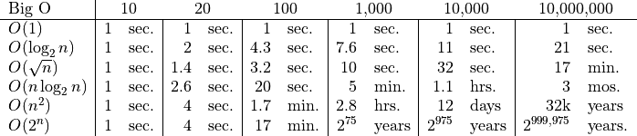
$\begin{tabular}{l|rl|rl|rl|rl|rl|rl} Big O & \multicolumn{2}{c}{10} & \multicolumn{2}{c}{20} & \multicolumn{2}{c}{100} & \multicolumn{2}{c}{1,000} & \multicolumn{2}{c}{10,000} & \multicolumn{2}{c}{10,000,000} \\ \hline $O(1)$ & 1 & sec. & 1 & sec. & 1 & sec. & 1 & sec. & 1 & sec. & 1 & sec. \\ $O(\log_2 n)$ & 1 & sec. & 2 & sec. & 4.3 & sec. & 7.6 & sec. & 11 & sec. & 21 & sec. \\ $O(\sqrt{n})$ & 1 & sec. & 1.4 & sec. & 3.2 & sec. & 10 & sec. & 32 & sec. & 17 & min. \\ $O(n \log_2 n)$ & 1 & sec. & 2.6 & sec. & 20 & sec. & 5 & min. & 1.1 & hrs. & 3 & mos. \\ $O(n^2)$ & 1 & sec. & 4 & sec. & 1.7 & min. & 2.8 & hrs. & 12 & days & 32k & years \\ $O(2^n)$ & 1 & sec. & 4 & sec. & 17 & min. & $2^{75}$ & years & $2^{975}$ & years & $2^{999,975}$ & years. \\ \end{tabular}$

(1 year is about $2^{25}$ seconds.)

Or, put another way, let’s say it takes $1 of memory to process 10 records. Here’s how much memory you would have to but to process a different number of records for different Big-O’s.

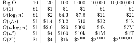
$\begin{tabular}{l|r|r|r|r|r|r} Big O & 10 & 20 & 100 & 1,000 & 10,000 & 10,000,000 \\ \hline $O(1)$ & \$1 & \$1 & \$1 & \$1 & \$1 & \$1 \\ $O(\log_2 n)$ & \$1 & \$2 & \$4.3 & \$7.6 & \$11 & \$21 \\ $O(\sqrt{n})$ & \$1 & \$1.4 & \$3.2 & \$10 & \$32 & \$1k \\ $O(n \log_2 n)$ & \$1 & \$2.6 & \$20 & \$300 & \$4k & \$7M \\ $O(n^2)$ & \$1 & \$4 & \$100 & \$10k & \$1M & \$1T \\ $O(2^n)$ & \$1 & \$4 & \$1k & $\$2^{100}$ & $\$2^{1,000}$ & $\$2^{1,000,000}$ \\ \end{tabular}$

I want to point out to you something you probably didn’t notice. The $O(\sqrt{n})$ is actually better than $O(\log_2 n)$ when we only double n. Sometimes people choose bad algorithms for small n because it gives better results. You’ll see in practice many fancy algorithms have available several different algorithms to use, and will switch algorithms based on the size of the data set. For smaller n, it will use less efficient algorithms that wouldn’t work well for larger n.

Formal Definition of Big O Notation¶

Mathematically, we say that $f(x) = O(g(x))$ as $x \rightarrow \infty$ when f(x) < Mg(x) for all $x \geq x_0$ . In other words, there is some number $M$ that you can multiply $g(x)$ by that is always larger than the corresponding $f(x)$ beyond some value of $x$ .

What this gives us is a function ( $g(x)$ ) that describes how $f(x)$ behaves as $x$ gets larger and larger, dropping any coefficient that really doesn’t help us understand the behavior.

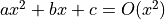
It’s rather trivial to convert $f(x)$ into $g(x)$ : Just keep the term that blows up the biggest and drop the coefficients.

Examples:

$a = O(1)$
$ax + b = O(x)$
$ax^2 + bx + c = O(x^2)$
$5\sqrt{x} + 27 \log_2 (15 x) - 181 = O(\sqrt(x))$

Properties of Big O Notation¶

Let’s now look at some properties of Big O.

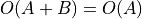$O(A + B) = O(A)$ when $A$ blows up faster. ( $O(B)$ otherwise.) Thus, we should never see Big O of sums.
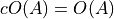$cO(A) = O(A)$ when $c$ is some constant number.
$A \cdot O(B) = O(A \cdot B)$

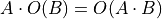
We Use Two Big O’s¶

There are two things we care about when we are looking at algorithms and judging how bad they get.

How long the algorithm takes to run.
How much memory it requires to run.

Since we can often trade memory for time, and time for memory, we should really consider both of these parameters. We’ll develop a separate Big O for each one.

How to Calculate Complexity of an Algorithm¶

Calculating Big O isn’t hard, but you have to be careful not to make a mistake, just like when you are solving math problems.

These are the general steps I use to calculate Big-O for time:

First, ignore all linear code. That is, if you have a chunk of code with no loops and no function calls, consider it a single line of code.
When calling a function, the Big O for that call is the same as the Big O for the function.
Next, when considering loops, count the number of times it will loop and consider each branch separately. If a loop has branches inside, one that calls a function and one that doesn’t, you’ll have to count the number of times it will call the function and the number of times it doesn’t.

To calculate it for memory, I look for the maximum amount of memory used to run the algorithm.

Each variable or slot of memory takes up 1 unit, no matter its actual size.
Each function call also takes up 1 slot of memory.
For recursive functions, we look at how deep it might go. (If we have tail recursion, it would be constant. But we don’t in Python, so we have to know how deep it will go.)
We should also consider how big the input and output is. IE, if you’re looking up a record in an array, then you have to store the records in memory in one shape or another.

Example 1: Recursive Fibonacci¶

Let’s do a few examples, using some recursive functions and some loops.

Calculating Big O for the Fibonacci involves us analyzing the code. Here is a simple version:

def fibonacci(n):
    if n <= 0: return 0
    elif n == 1: return 1
    else: return fibonacci(n-1) + fibonacci(n-2)

We’re going to calculate this by calculating the number of function calls based on the parameter n. We’ll call this function $F(n)$ .

If n<=1, then 1 call is made. $F(0) = F(1) = 1$ .

If n==2, then we have 3 calls: 1 for 2, 1 for 1, and another for 0. $F(2) = 1 + F(1) + F(0) = 3$

If n==3, then we have 5 calls: 1 for 3, 3 for 2, and 1 for 1. $F(3) = 1 + F(2) = F(1) = 5$ .

For any n>1, we have the formula F(n) = 1 + F(n-1) + F(n-2), which itself is a kind of Fibonacci sequence.

We’ll use Proof by Induction to calculate F. If you haven’t seen my Basic Mathematics video on Proof by Induction, you can watch it later.

Here’s how proof by induction works. First, we make up an answer. Then, we prove that the answer works for $n=1$ . Then we prove that the answer works for $n+1$ , assuming it works for $n$ .

Let’s assume that recursive fibonacci is exponential: $F(n)=a^{n-1}$ .

We’re skipping n=0. It’s just 1 anyway, which will be lost in Big O notation.

This works for $n=1$ as $a^0=1$ .

What about for $n+1$ ?

$\begin{aligned} F(n+1) &= a^n && \text{We want to prove this. Maybe we can find }a{?} \\ F(n+1) &= 1 + F(n) + F(n-1) \\ F(n) &= a^{n-1} && \text{We are assuming this is true.} \\ F(n-1) &= a^{n-2} && \text{Also assumed.} \\ a^{n} &= 1 + a^{n-1} + a^{n-2} && \text{We must prove this true.} \\ a^{2} &= \frac{1}{a^{n-2}} + a + 1 && \text{Divide by } a^{n-2} \\ a^{2} &= a + 1 && n \rightarrow \infty\\ a &= \frac{1 + \sqrt{5}}{2} = \phi && \text{Only interested in }a>1\\ \end{aligned}$

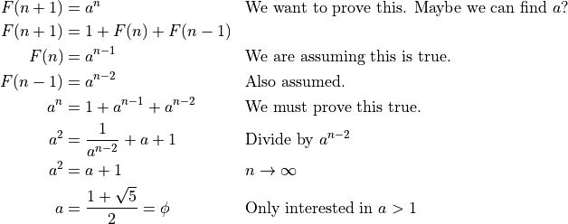
$\phi$ is the Golden Ratio, about 1.618.

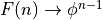So, as $n \rightarrow \infty$ , $F(n) \rightarrow \phi^{n-1}$ .

We’ll use 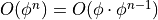$O(\phi^n)=O(\phi \cdot \phi^{n-1})$ to drop the useless $-1$ . That’s how much time it will take to calculate the Fibonacci element for large n. This is quite bad, and I don’t recommend doing it for anything other than a learning exercise.

How much memory does recursive fibonacci use? The answer is rather easy. At most, it will have n frames on the stack. So it is $O(n)$ .

Example: Fibonacci Loop¶

Let’s examine the Fibonacci loop.

def fibonacci(n):
    if n <= 0: return 0
    if n == 1: return 1
    prev_prev = 0
    prev = 1
    while n > 1:
        result = prev + prev_prev
        prev_prev = prev
        prev = result
        n = n - 1
    return result

How many times do we need to iterate through the loop? The answer is simple: n times! Since there are no function calls or branches inside the loop, there is nothing more to consider. This function is $O(n)$ . This is significantly better than the previous recursive implementation, but it is still not very good for calculating very large n.

The memory usage of this algorithm, however, is excellent. It doesn’t matter how large n is, it will always use the same three variables, and never make any function calls. So it is $O(1)$ in terms of memory.

Example: Cached Fibonacci¶

Can we do better? We could possibly store the first million terms of the Fibonacci sequence in memory, trading speed for memory. Each term would be an integer, possibly quite large, but as long as n isn’t too big, it would be O(n) to store the first n terms in memory. But it will be very fast! O(1) in fact to retrieve any of thise first n terms!

Perhaps you can store only two adjacent terms spread out. So you store fibonacci(100) and fibonacci(101), and then if you want to calculate fibonacci(102) you just look up the previous two terms. This would reduce the amount of memory required by how far you space them apart. But this would only reduce them by a fraction, so it is still $O(n)$ in memory. Calculating would still only take $O(1)$ time, since at most you’d have to calculate 98 terms for any n.

This is an example where what seems like a brilliant optimization doesn’t really solve the problem at hand. If you’re going to store some fraction of the fibonacci series in memory, then you’re getting O(1) time and O(n) memory usage.

Perhaps you want to spread out the terms that are stored in memory as n increases. You could get square root or logarithmic memory in such a case, but that would increase the amount of time from constant to logarithmic or square root or something like that.

Depending on what you intend to do with it, how much time you have, and how much memory you are willing to buy, you’ll have to find the right trade off.

More Possibilities¶

Or we can find better algorithms. (Look up Linear Recurrence if you’re interested.)

Or we can calculate estimates using even more math.

Conclusion¶

People poo-poo Big-O notation as some sort of interview exercise that’s used to keep people out of the industry. The truth is, I used Big-O all the time on my job. I had to know what the behavior of different algorithms were, debate with my colleagues about the merits of one algorithm versus another, and find new algorithms. We would often have discussions in the halls where we compared Big-O for various algorithms, and when you’re sifting through hundreds of possibilities and variations, being able to quickly find the Big-O of an algorithm, both for time and memory, was incredibly important.

If you want to work on my team, I’m going to ask you to learn Big-O and use it all the time. I’m going to ask you to describe the Big-O for the code you intend to write, and I’m going to expect you to check that I’m not making a miscalculation.

So don’t just study this to pass the interview. Study it to become a great software developer.

In the upcoming videos, I’m going to refer back to Big-O a lot as an explanation for why we do things the way we do.